Optional Module 8 Lab 3: Automated Enrichment and Visualisation Lab using `clusterProfiler`

This work is licensed under a Creative Commons Attribution-ShareAlike 3.0 Unported License. This means that you are able to copy, share and modify the work, as long as the result is distributed under the same license.

By Chaitra Sarathy

`clusterProfiler` lab

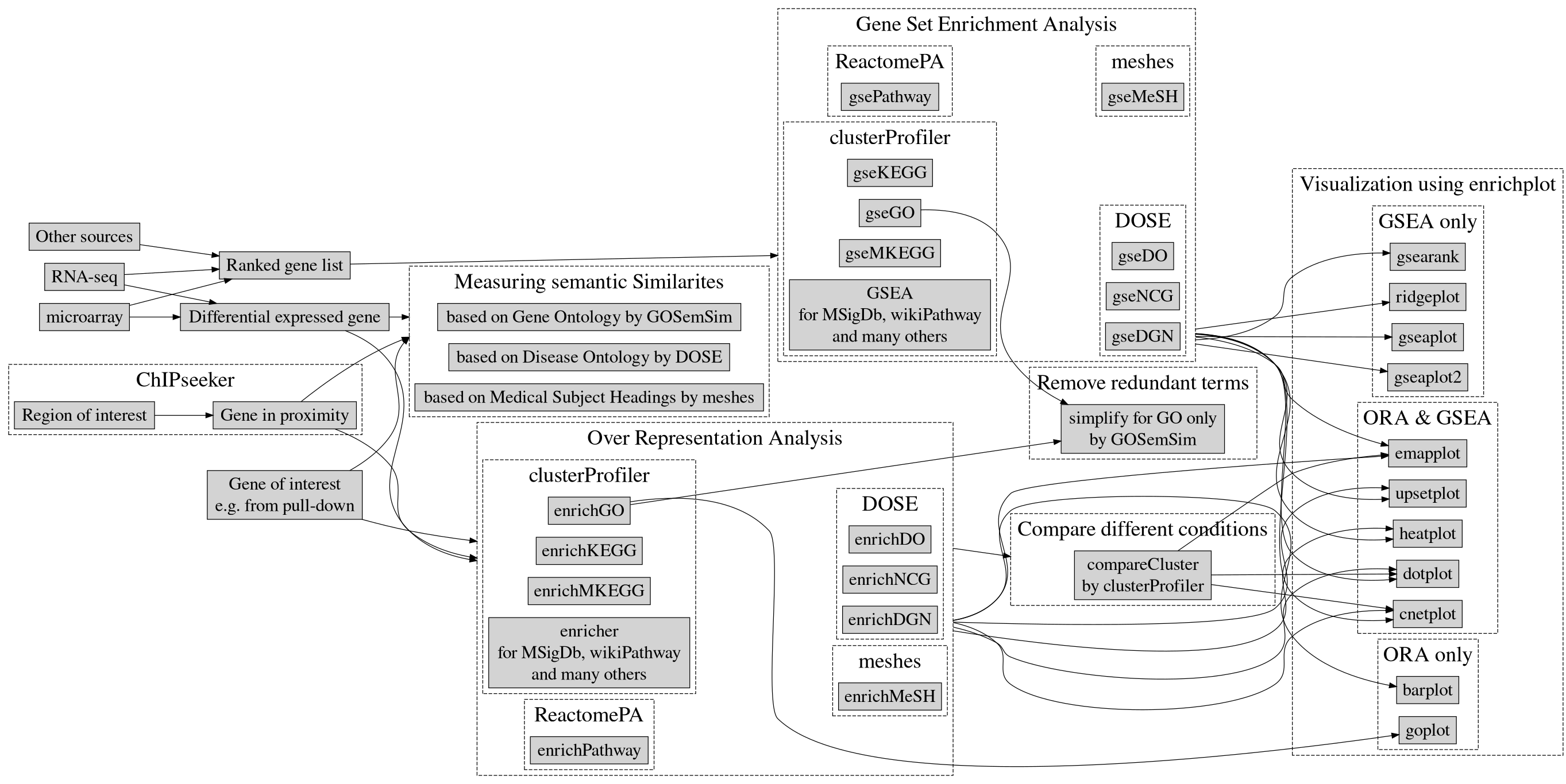
clusterProfiler is an R package that implements methods to perform both functional annotation and visualization of genes and gene clusters.

It can accept data from a variety of experimental sources such as DNA-seq, RNA-seq, microarray, Mass spectometry, meRIP-seq, m6A-seq, ATAC-seq and ChIP-seq and thus can be applied in diverse scenarios.
It provides a tidy interface to access, manipulate, and visualize enrichment results to help users achieve efficient data interpretation.

clusterProfiler is released within the Bioconductor project and the source code is hosted on GitHub.

Goal

Learn how to write R scripts for going from gene list to enriched pathways
Learn how to run over representation analysis (ORA) and gene set enrichment analysis (GSEA) using functions in the clusterProfiler R package
Explore results of enrichment analysis using various visualisation options in clusterProfiler

Supported Analysis

For functional annotation, clusterprofiler provides R functions to perform

Over Representation Analysis
Gene Set Enrichment Analysis
Biological theme comparison

In this practical, we will be learning how to run Over Representation Analysis and Gene Set Enrichment Analysis in 2 exercises. Follow the step-by-step checklist.

Before starting the exercises, make sure that clusterProfiler and other required packages are installed and loaded. Run “prework_module8_clusterprofiler.R” before following this module.

Install and load packages

To run enrichment analysis using clusterProfiler, we need a few additional packages org.Hs.eg.db, DOSE, tidyverse, enrichplot, ggupset. Install and load all necessary packages using this code:

# install and load the package  manager
if (!requireNamespace("BiocManager", quietly = TRUE))
  install.packages("BiocManager")

# list the required bioconductor packages 
bio.pkgs = c("clusterProfiler", "org.Hs.eg.db", "DOSE", "tidyverse", "enrichplot", "ggupset")

# install
BiocManager::install(bio.pkgs)

## 'getOption("repos")' replaces Bioconductor standard repositories, see
## 'help("repositories", package = "BiocManager")' for details.
## Replacement repositories:
##     CRAN: https://p3m.dev/cran/__linux__/jammy/latest

## Bioconductor version 3.19 (BiocManager 1.30.23), R 4.4.0 (2024-04-24)

## Warning: package(s) not installed when version(s) same as or greater than current; use
##   `force = TRUE` to re-install: 'clusterProfiler' 'org.Hs.eg.db' 'DOSE'
##   'tidyverse' 'enrichplot' 'ggupset'

## Installation paths not writeable, unable to update packages
##   path: /usr/local/lib/R/library
##   packages:
##     foreign, KernSmooth, MASS, nlme, survival

## Old packages: 'BiocNeighbors', 'BiocStyle', 'Biostrings', 'cli', 'crayon',
##   'DBI', 'digest', 'downlit', 'dqrng', 'evaluate', 'filehash', 'GenomicRanges',
##   'GSVA', 'KEGGREST', 'knitr', 'limma', 'locfit', 'markdown', 'PKI',
##   'RcppArmadillo', 'reticulate', 'rlang', 'rsconnect', 'scater', 'secretbase',
##   'SparseM', 'spatstat.data', 'spatstat.sparse', 'spatstat.utils', 'targets',
##   'xfun', 'XML', 'xts'

# load all at once
invisible(lapply(bio.pkgs, function(x) library(x, character.only=TRUE, quietly = T)))

##

## clusterProfiler v4.12.0  For help: https://yulab-smu.top/biomedical-knowledge-mining-book/
## 
## If you use clusterProfiler in published research, please cite:
## T Wu, E Hu, S Xu, M Chen, P Guo, Z Dai, T Feng, L Zhou, W Tang, L Zhan, X Fu, S Liu, X Bo, and G Yu. clusterProfiler 4.0: A universal enrichment tool for interpreting omics data. The Innovation. 2021, 2(3):100141

## 
## Attaching package: 'clusterProfiler'

## The following object is masked from 'package:stats':
## 
##     filter

## 
## Attaching package: 'BiocGenerics'

## The following objects are masked from 'package:stats':
## 
##     IQR, mad, sd, var, xtabs

## The following objects are masked from 'package:base':
## 
##     anyDuplicated, aperm, append, as.data.frame, basename, cbind,
##     colnames, dirname, do.call, duplicated, eval, evalq, Filter, Find,
##     get, grep, grepl, intersect, is.unsorted, lapply, Map, mapply,
##     match, mget, order, paste, pmax, pmax.int, pmin, pmin.int,
##     Position, rank, rbind, Reduce, rownames, sapply, setdiff, table,
##     tapply, union, unique, unsplit, which.max, which.min

## Welcome to Bioconductor
## 
##     Vignettes contain introductory material; view with
##     'browseVignettes()'. To cite Bioconductor, see
##     'citation("Biobase")', and for packages 'citation("pkgname")'.

## 
## Attaching package: 'S4Vectors'

## The following object is masked from 'package:clusterProfiler':
## 
##     rename

## The following object is masked from 'package:utils':
## 
##     findMatches

## The following objects are masked from 'package:base':
## 
##     expand.grid, I, unname

## 
## Attaching package: 'IRanges'

## The following object is masked from 'package:clusterProfiler':
## 
##     slice

## 
## Attaching package: 'AnnotationDbi'

## The following object is masked from 'package:clusterProfiler':
## 
##     select

##

## DOSE v3.30.1  For help: https://yulab-smu.top/biomedical-knowledge-mining-book/
## 
## If you use DOSE in published research, please cite:
## Guangchuang Yu, Li-Gen Wang, Guang-Rong Yan, Qing-Yu He. DOSE: an R/Bioconductor package for Disease Ontology Semantic and Enrichment analysis. Bioinformatics 2015, 31(4):608-609

## ── Attaching core tidyverse packages ──────────────────────── tidyverse 2.0.0 ──
## ✔ dplyr     1.1.4     ✔ readr     2.1.5
## ✔ forcats   1.0.0     ✔ stringr   1.5.1
## ✔ ggplot2   3.5.1     ✔ tibble    3.2.1
## ✔ lubridate 1.9.3     ✔ tidyr     1.3.1
## ✔ purrr     1.0.2     
## ── Conflicts ────────────────────────────────────────── tidyverse_conflicts() ──
## ✖ lubridate::%within%() masks IRanges::%within%()
## ✖ dplyr::collapse()     masks IRanges::collapse()
## ✖ dplyr::combine()      masks Biobase::combine(), BiocGenerics::combine()
## ✖ dplyr::desc()         masks IRanges::desc()
## ✖ tidyr::expand()       masks S4Vectors::expand()
## ✖ dplyr::filter()       masks clusterProfiler::filter(), stats::filter()
## ✖ dplyr::first()        masks S4Vectors::first()
## ✖ dplyr::lag()          masks stats::lag()
## ✖ ggplot2::Position()   masks BiocGenerics::Position(), base::Position()
## ✖ purrr::reduce()       masks IRanges::reduce()
## ✖ dplyr::rename()       masks S4Vectors::rename(), clusterProfiler::rename()
## ✖ lubridate::second()   masks S4Vectors::second()
## ✖ lubridate::second<-() masks S4Vectors::second<-()
## ✖ dplyr::select()       masks AnnotationDbi::select(), clusterProfiler::select()
## ✖ purrr::simplify()     masks clusterProfiler::simplify()
## ✖ dplyr::slice()        masks IRanges::slice(), clusterProfiler::slice()
## ℹ Use the conflicted package (<http://conflicted.r-lib.org/>) to force all conflicts to become errors

Once all packages are loaded, we can get started with exercises.

Exercise 1a. Over representation analysis

clusterProfiler supports over representation analysis against various sources such as GO annotation, KEGG pathway, MSigDB to name a few. For the full list please refer this link.

In this exercise, we will learn over representation analysis using the gene ontology annotations. This is implemented in the function enrichGO().

Data for enrichment using `clusterProfiler`

Let us start with loading the dataset geneList that is provided by the package DOSE.

DOSE provides an example dataset geneList. It comes from analysis of a breast cancer dataset that had 200 samples, including 29 samples in grade I, 136 samples in grade II and 35 samples in grade III. The ratios of geometric means of grade III samples versus geometric means of grade I samples were computed. Logarithm of these ratios (base 2) are stored in geneList dataset.

data(geneList, package="DOSE")

A variable called geneList should be loaded in your R environment. What does it look like?

head(geneList)

##     4312     8318    10874    55143    55388      991 
## 4.572613 4.514594 4.418218 4.144075 3.876258 3.677857

As you can see, first line of output has names of genes in Entrez gene ID format and the second line has fold change values of genes.

Data for over representation analysis using `clusterProfiler`

For running an over representation analysis, we need only a list of gene names or IDs. Let us extract out the genes which had an expression value >2 or <-2 using the function names()

gene <- names(geneList)[abs(geneList) > 2]

head(gene)

## [1] "4312"  "8318"  "10874" "55143" "55388" "991"

gene has a list of 207 genes.

Perform GO over representation analysis

Now, run enrichGO() with this list of genes and examine the results

ego <- enrichGO(gene          = gene,
                universe      = names(geneList),
                OrgDb         = org.Hs.eg.db,
                ont           = "ALL",
                pAdjustMethod = "BH",
                pvalueCutoff  = 0.01,
                qvalueCutoff  = 0.05,
                readable      = TRUE)

Results of GO over representation analysis

Examine the results. Do you notice any similarities or differences between this output format and your results from Module 2 gProfiler?

The output table is stored in ego@result. In this example, 152 processes were significantly enriched.

head(ego)

##            ONTOLOGY         ID                          Description GeneRatio
## GO:0098813       BP GO:0098813       nuclear chromosome segregation    34/197
## GO:0000070       BP GO:0000070 mitotic sister chromatid segregation    28/197
## GO:0000819       BP GO:0000819         sister chromatid segregation    30/197
## GO:0140014       BP GO:0140014             mitotic nuclear division    32/197
## GO:0007059       BP GO:0007059               chromosome segregation    37/197
## GO:0000280       BP GO:0000280                     nuclear division    37/197
##              BgRatio       pvalue     p.adjust       qvalue
## GO:0098813 238/11586 3.730986e-22 1.124892e-18 1.034858e-18
## GO:0000070 152/11586 1.909540e-21 2.878631e-18 2.648230e-18
## GO:0000819 185/11586 3.017475e-21 3.032563e-18 2.789841e-18
## GO:0140014 224/11586 7.008600e-21 4.403280e-18 4.050849e-18
## GO:0007059 319/11586 7.302289e-21 4.403280e-18 4.050849e-18
## GO:0000280 327/11586 1.726930e-20 8.677821e-18 7.983262e-18
##                                                                                                                                                                                                                                  geneID
## GO:0098813                     CDCA8/CDC20/KIF23/CENPE/MYBL2/CCNB2/NDC80/TOP2A/NCAPH/ASPM/DLGAP5/UBE2C/SKA1/NUSAP1/TPX2/TACC3/NEK2/CDK1/MAD2L1/KIF18A/CDT1/BIRC5/KIF11/TTK/NCAPG/AURKB/TRIP13/PRC1/KIFC1/KIF18B/AURKA/CCNB1/KIF4A/PTTG1
## GO:0000070                                                        CDCA8/CDC20/KIF23/CENPE/MYBL2/NDC80/NCAPH/DLGAP5/UBE2C/SKA1/NUSAP1/TPX2/NEK2/CDK1/MAD2L1/KIF18A/CDT1/BIRC5/KIF11/TTK/NCAPG/AURKB/TRIP13/PRC1/KIFC1/KIF18B/CCNB1/KIF4A
## GO:0000819                                            CDCA8/CDC20/KIF23/CENPE/MYBL2/NDC80/TOP2A/NCAPH/DLGAP5/UBE2C/SKA1/NUSAP1/TPX2/TACC3/NEK2/CDK1/MAD2L1/KIF18A/CDT1/BIRC5/KIF11/TTK/NCAPG/AURKB/TRIP13/PRC1/KIFC1/KIF18B/CCNB1/KIF4A
## GO:0140014                                 CDCA8/CDC20/KIF23/CENPE/MYBL2/NDC80/NCAPH/DLGAP5/UBE2C/SKA1/NUSAP1/TPX2/NEK2/UBE2S/CDK1/MAD2L1/KIF18A/CDT1/BIRC5/KIF11/TTK/NCAPG/AURKB/CHEK1/TRIP13/PRC1/KIFC1/KIF18B/AURKA/CCNB1/KIF4A/BMP4
## GO:0007059   CDCA8/CDC20/KIF23/CENPE/MYBL2/CCNB2/NDC80/TOP2A/NCAPH/ASPM/DLGAP5/UBE2C/HJURP/SKA1/NUSAP1/TPX2/TACC3/NEK2/CENPM/CENPN/CDK1/MAD2L1/KIF18A/CDT1/BIRC5/KIF11/TTK/NCAPG/AURKB/TRIP13/PRC1/KIFC1/KIF18B/AURKA/CCNB1/KIF4A/PTTG1
## GO:0000280 CDCA8/CDC20/KIF23/CENPE/MYBL2/CCNB2/NDC80/TOP2A/NCAPH/ASPM/DLGAP5/UBE2C/SKA1/NUSAP1/TPX2/NEK2/RAD51AP1/UBE2S/CDK1/MAD2L1/KIF18A/CDT1/BIRC5/KIF11/TTK/NCAPG/AURKB/CHEK1/TRIP13/PRC1/KIFC1/KIF18B/AURKA/CCNB1/KIF4A/PTTG1/BMP4
##            Count
## GO:0098813    34
## GO:0000070    28
## GO:0000819    30
## GO:0140014    32
## GO:0007059    37
## GO:0000280    37

nrow(ego@result)

## [1] 152

Input options for `enrichGO()`:

The default option for gene is entrez gene ID, but other gene ID formats are supported in GO analyses. You should specify the keyType parameter to specify the input gene ID type (More details below)
We have selected all genes measured in the experiment as our universe.
You can specify subontology using the argument ont. It takes one option among - “BP”, “MF”, “CC” or “ALL” for biological process, molecular function, cellular co-localization or all subontologies respectively.
If readable is set to TRUE, the input gene IDs will be converted to gene symbols.
OrgDb is the genome annotation database of organism that your gene list is coming from. Since our geneList is from human breast cancer, we have provided human OrgDb object (org.Hs.eg.db). See the section “A note on supported organisms” for more details.

Gene IDs can be converted to different formats using bitr() function.

# convert from entrez gene ID to ensembl ID and gene symbols
gene.df <- bitr(gene, 
                fromType = "ENTREZID",
                toType = c("ENSEMBL", "SYMBOL"),
                OrgDb = org.Hs.eg.db)

## 'select()' returned 1:many mapping between keys and columns

## Warning in bitr(gene, fromType = "ENTREZID", toType = c("ENSEMBL", "SYMBOL"), :
## 0.48% of input gene IDs are fail to map...

head(gene.df)

##   ENTREZID         ENSEMBL SYMBOL
## 1     4312 ENSG00000196611   MMP1
## 2     8318 ENSG00000093009  CDC45
## 3    10874 ENSG00000109255    NMU
## 4    55143 ENSG00000134690  CDCA8
## 5    55388 ENSG00000065328  MCM10
## 6      991 ENSG00000117399  CDC20

Various options for keyType can be found using keytypes(<name of organism annotation>). For example: keytypes(org.Hs.eg.db)

Simplify `enrichGO()` results

GO enrichment typically contains redundant terms. You may use the simplify() function to reduce redundancy of enriched GO terms using the default parameters. Please note that simplifying is not always a necessary step. You can choose to omit it, based on the nature of your result tables.

ego.sim = clusterProfiler::simplify(ego)
nrow(ego.sim)

## [1] 46

Exercise 1b. Visualise the results of GO over representation analysis

Barplot

Bar plot is the most widely used method to visualize enriched terms. It shows the enrichment scores (e.g. p values) and gene count or ratio as bar height and color. You can specify the number of terms (most significant) to display via the showCategory parameter.

barplot(ego.sim, showCategory=20) + ggtitle("ORA barplot (top 20)")

You can plot other variables such as log10(p.adjust) by modifying using mutate() from the tidyverse package

mutate(ego.sim, qscore = -log(p.adjust, base=10)) %>% 
    barplot(x="qscore", showCategory=20) + ggtitle("ORA barplot - qvalue (top 20)")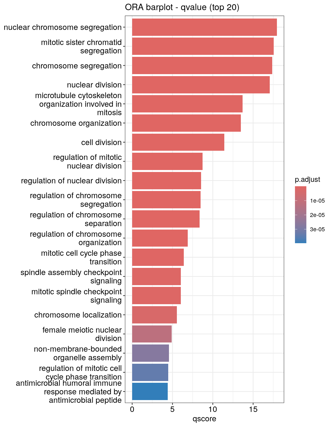

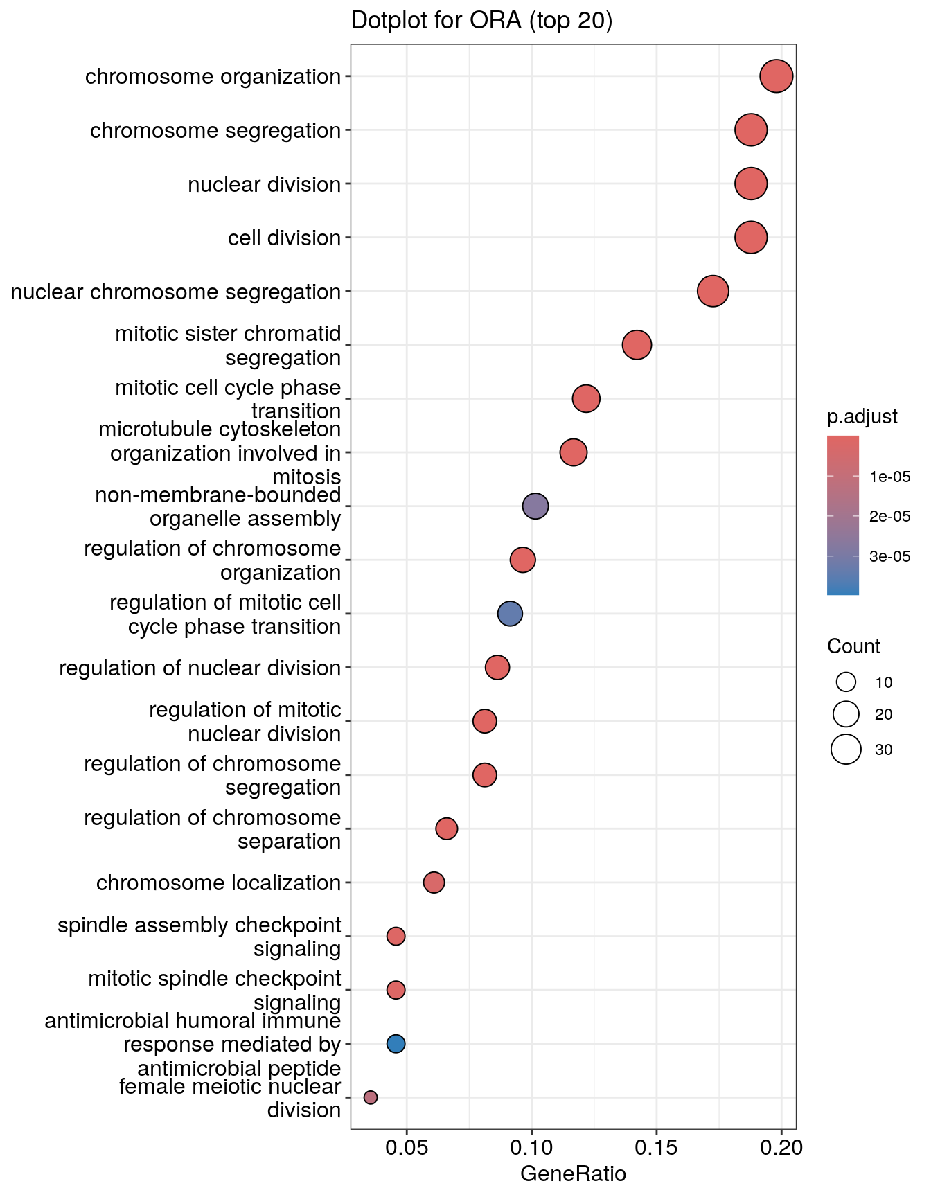
Dotplot

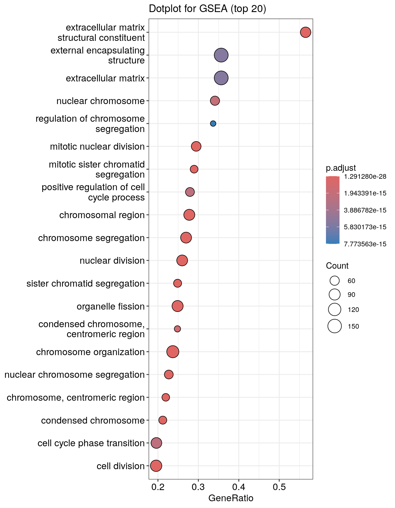
Dot plot is very similar to bar plot. It has additional capability to encode another score as dot size.

dotplot(ego.sim, showCategory=20) + ggtitle("Dotplot for ORA (top 20)")

Enrichment Map

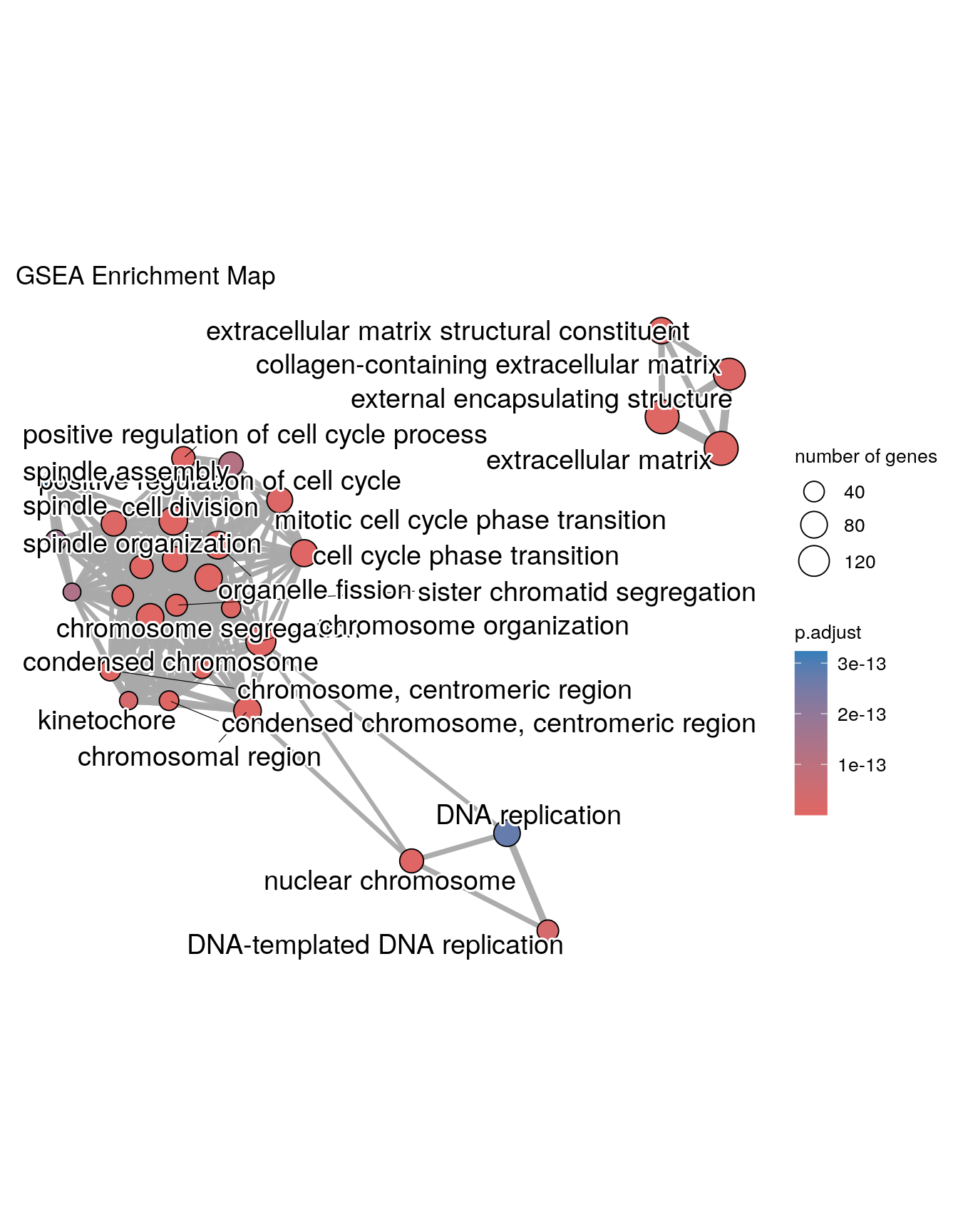
Enrichment map organizes enriched terms into a network with edges connecting overlapping gene sets. In this way, mutually overlapping gene sets are tend to cluster together, making it easy to identify functional module. Before making the map, similarity must be calculated. This can be done using pairwise_termsim()

edo <- pairwise_termsim(ego.sim)
emapplot(edo)+ ggtitle("ORA Enrichment Map")

## Warning: ggrepel: 6 unlabeled data points (too many overlaps). Consider
## increasing max.overlaps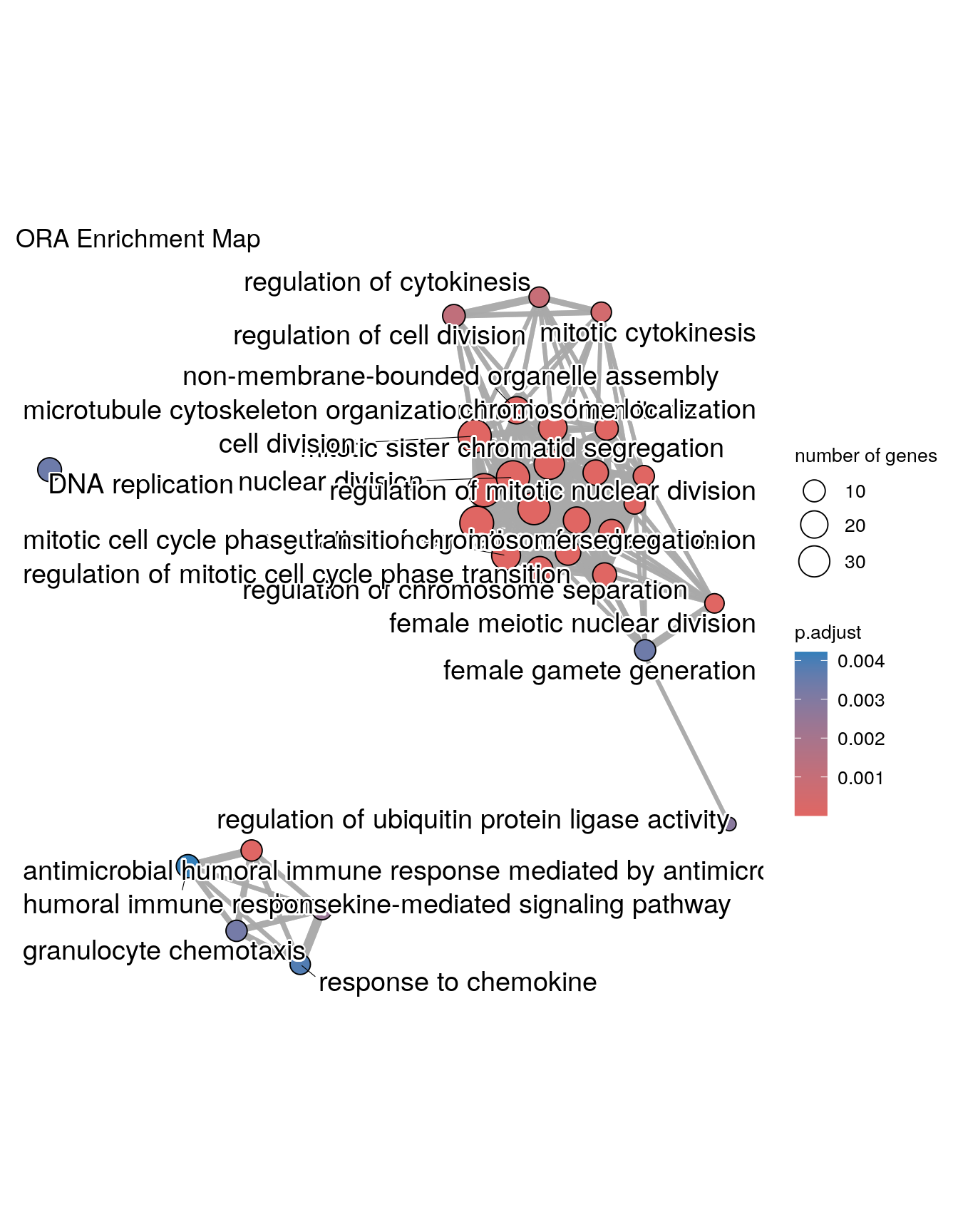

Upset plot

The upsetplot is for visualizing the complex association between genes and gene sets. It emphasizes the gene overlapping among different gene sets.

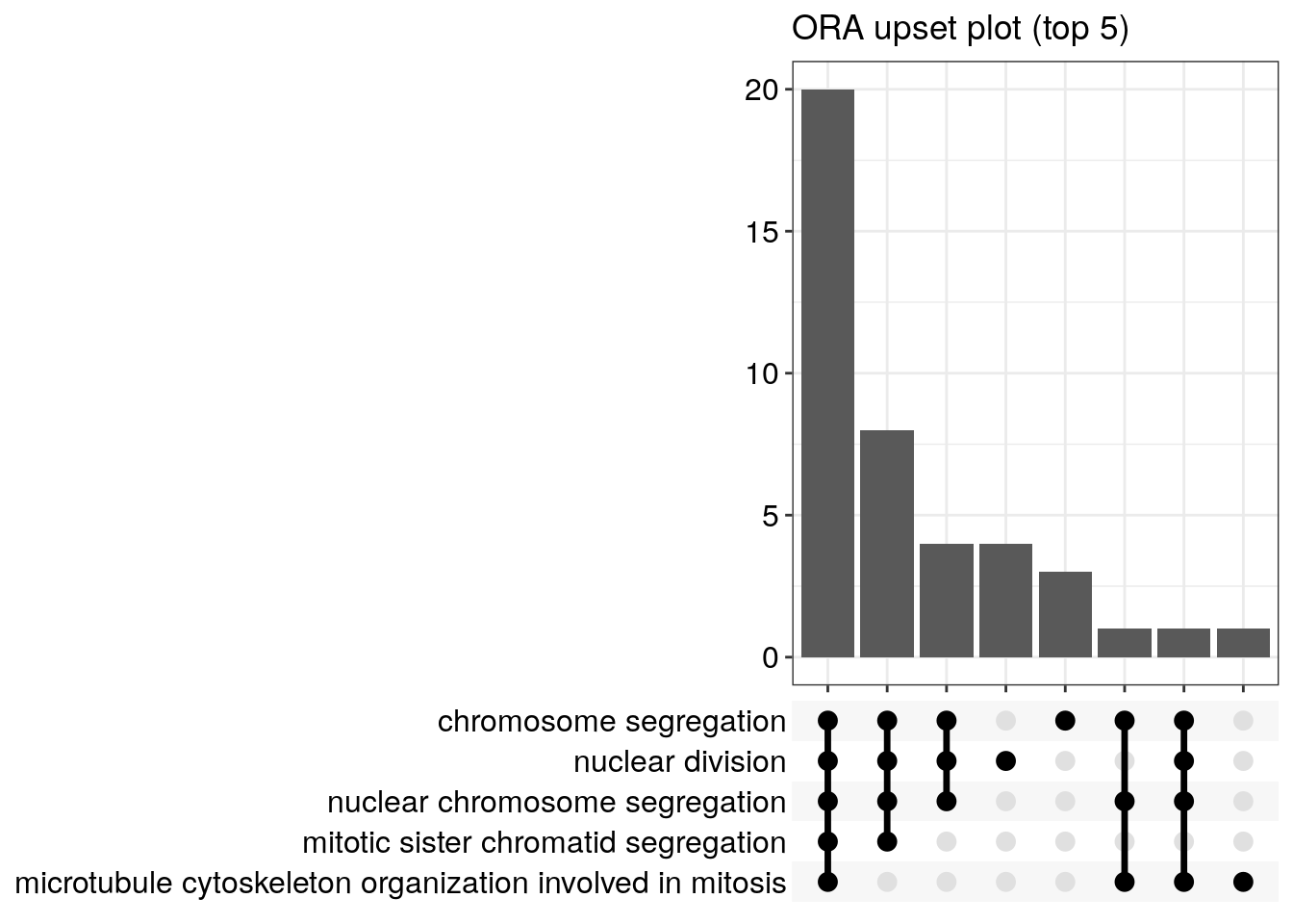
upsetplot(edo, n=5) + ggtitle("ORA upset plot (top 5)")

Details about the input arguments for `enrichGO()`

gene a vector of entrez gene ID. OrgDb OrgDb object keyType keytype of input gene ont One of “BP”, “MF”, and “CC” subontologies, or “ALL” for all three pvalueCutoff adjusted pvalue cutoff on enrichment tests to report pAdjustMethod one of “holm”, “hochberg”, “hommel”, “bonferroni”, “BH”, “BY”, “fdr”, “none” universe background genes. If missing, the all genes listed in the database (eg TERM2GENE table) will be used as background qvalueCutoff qvalue cutoff on enrichment tests to report as significant. Tests must pass i) pvalueCutoff on unadjusted pvalues, ii) pvalueCutoff on adjusted pvalues and iii) qvalueCutoff on qvalues to be reported minGSSize minimal size of genes annotated by Ontology term for testing maxGSSize maximal size of genes annotated for testing readable whether mapping gene ID to gene Name

A note on supported organisms

GO analyses in clusterProfiler support organisms that have an OrgDb object available. OrgDb (organism databases) objects are databases that contain genome annotations and thus, they are best for converting gene IDs or obtaining GO information for current genome builds.A list of organism databases can be found here

Exercise 2a: Gene set enrichment analysis

Data for running gene set enrichment analysis in `clusterProfiler`

GSEA analysis requires a ranked gene list, which contains three features:

numeric vector: fold change or other type of numerical variable
named vector: every number has a name, the corresponding gene ID
sorted vector: number should be sorted in decreasing order

Since geneList is already in the desired format, we will use it for this exercise. If you haven’t loaded it, use the command below to import the data. Please see the above section “Data for enrichment using clusterProfiler” for details regarding the dataset.

data(geneList, package="DOSE")
head(geneList)

##     4312     8318    10874    55143    55388      991 
## 4.572613 4.514594 4.418218 4.144075 3.876258 3.677857

Perform GO gene set enrichment analysis

The clusterProfiler package provides the gseGO() function for gene set enrichment analysis using gene ontology. You can run GSEA as below:

set.seed(100)
egsea <- gseGO(geneList     = geneList,
               OrgDb        = org.Hs.eg.db,
               ont          = "ALL",
               minGSSize    = 100,
               maxGSSize    = 500,
               pvalueCutoff = 0.05,
               pAdjustMethod = "BH",
               eps = 0,
               verbose      = FALSE)

Results of GO gene set enrichment analysis

Examine the results. Do you notice any similarities or differences between this output format and your results from Module 2 GSEA?

The output table is stored in egsea@result. In this example, 512 processes were significantly enriched.

head(egsea)

##            ONTOLOGY         ID                          Description setSize
## GO:0051276       BP GO:0051276              chromosome organization     473
## GO:0098813       BP GO:0098813       nuclear chromosome segregation     238
## GO:0007059       BP GO:0007059               chromosome segregation     319
## GO:0000819       BP GO:0000819         sister chromatid segregation     185
## GO:0000070       BP GO:0000070 mitotic sister chromatid segregation     152
## GO:0000280       BP GO:0000280                     nuclear division     327
##            enrichmentScore      NES       pvalue     p.adjust       qvalue rank
## GO:0051276       0.5201824 2.544408 9.093519e-32 1.291280e-28 7.676844e-29 1374
## GO:0098813       0.6333337 2.877824 3.191110e-30 1.768253e-27 1.051252e-27  449
## GO:0007059       0.5847891 2.734065 3.735745e-30 1.768253e-27 1.051252e-27 1374
## GO:0000819       0.6606162 2.927964 4.701535e-27 1.669045e-24 9.922713e-25  449
## GO:0000070       0.6861425 2.972105 5.809969e-26 1.650031e-23 9.809674e-24  532
## GO:0000280       0.5414575 2.545927 5.146366e-25 1.217973e-22 7.241027e-23 1246
##                              leading_edge
## GO:0051276 tags=24%, list=11%, signal=22%
## GO:0098813  tags=23%, list=4%, signal=22%
## GO:0007059 tags=27%, list=11%, signal=25%
## GO:0000819  tags=25%, list=4%, signal=24%
## GO:0000070  tags=29%, list=4%, signal=28%
## GO:0000280 tags=26%, list=10%, signal=24%
##                                                                                                                                                                                                                                                                                                                                                                                                                                                                                                                                                                                                             core_enrichment
## GO:0051276 8318/55143/991/9493/1062/4605/10403/7153/23397/9787/11065/55355/220134/51203/22974/10460/4751/55839/983/4085/9837/81930/81620/332/3832/2146/7272/64151/9212/51659/9319/9055/3833/146909/891/24137/4174/9232/4171/9928/11004/990/5347/29127/26255/701/9156/11130/57405/10615/3159/79075/2491/8438/9700/5888/898/3149/11339/9134/4175/4173/2237/22948/5984/9918/1058/84296/2643/699/4609/1063/5111/64785/9401/26271/55055/641/1763/54892/8357/3024/4176/3148/3006/4436/5982/9735/908/23310/8607/3008/10051/10576/3009/4172/9631/83990/5885/11200/2072/84722/51115/7283/5983/4678/5588/54908/10592/51377/4683/54069
## GO:0098813                                                                                                                                                                                                                                                                                                                   55143/991/9493/1062/4605/9133/10403/7153/23397/259266/9787/11065/220134/51203/22974/10460/4751/983/4085/81930/81620/332/3832/7272/64151/9212/9319/9055/3833/146909/6790/891/24137/9232/9928/11004/990/5347/29127/26255/701/11130/57405/10615/1894/2491/9700/898/9134/9918/699/1063/26271/55055
## GO:0007059                                                                                                                            55143/991/9493/1062/4605/9133/10403/7153/23397/259266/9787/11065/55355/220134/51203/22974/10460/4751/79019/55839/983/4085/81930/81620/332/3832/7272/64151/9212/9319/9055/3833/146909/6790/891/24137/9232/9928/11004/990/5347/29127/26255/701/11130/79682/57405/10615/1894/2491/9700/898/11339/4288/54801/9134/29899/9918/699/6491/1063/26271/55055/54892/29901/79980/9735/55732/81624/23310/292/10051/1104/5359/83990/5885/11200/203068/84722/51115/7283/51647/54908/10592/6732/54069
## GO:0000819                                                                                                                                                                                                                                                                                                                                                             55143/991/9493/1062/4605/10403/7153/23397/9787/11065/220134/51203/22974/10460/4751/983/4085/81930/81620/332/3832/7272/64151/9212/9319/9055/3833/146909/891/24137/9928/11004/990/5347/29127/701/11130/57405/10615/2491/9700/9918/699/1063/26271/55055
## GO:0000070                                                                                                                                                                                                                                                                                                                                                                      55143/991/9493/1062/4605/10403/23397/9787/11065/220134/51203/22974/4751/983/4085/81930/81620/332/3832/7272/64151/9212/9319/9055/3833/146909/891/24137/9928/11004/5347/29127/701/11130/57405/10615/2491/9700/9918/699/1063/26271/55055/54892
## GO:0000280                                                                                                                                              55143/991/9493/1062/4605/9133/10403/7153/23397/259266/9787/11065/220134/51203/22974/4751/10635/27338/983/4085/81930/81620/332/3832/7272/64151/9212/1111/9319/9055/3833/146909/6790/891/24137/9232/9928/1164/11004/4603/5347/29127/26255/701/11130/57405/10615/2491/8438/9700/5888/898/4288/9134/2175/91646/994/9918/699/1063/26271/55055/54892/5902/9585/9735/23310/2253/8877/9088/995/10051/79703/1104/79866/83990/5885/11200/2072/940/1761/84722/51115/7283/80010

nrow(egsea@result)

## [1] 517

Input options for `gseGO()`

Note that only gene sets having the size within [minGSSize, maxGSSize] will be tested.
Similar to enrichGO(), you can specify subontology using the argument ont. It takes one option among - “BP”, “MF”, “CC” or “ALL” for biological process, molecular function, cellular co-localization or all subontologies respectively
pvalueCutoff defines the cutoff for pvalue that is used for determining significant processes
Setting eps to zero improves estimation.
pAdjustMethod can be one of “holm”, “hochberg”, “hommel”, “bonferroni”, “BH”, “BY”, “fdr”, “none”

Details about the input arguments for `gseGO()`

geneList order ranked geneList ont one of “BP”, “MF”, and “CC” subontologies, or “ALL” for all three OrgDb OrgDb keyType keytype of gene exponent weight of each step minGSSize minimal size of each geneSet for analyzing maxGSSize maximal size of genes annotated for testing eps This parameter sets the boundary for calculating the p value pvalueCutoff pvalue Cutoff pAdjustMethod pAdjustMethod one of “holm”, “hochberg”, “hommel”, “bonferroni”, “BH”, “BY”, “fdr”, “none” verbose print message or not seed logical by one of ‘fgsea’ or ‘DOSE’

Exercise 2b. Visualise the results of gene set enrichment analysis

Dotplot

You can use the function dotplot() to summarise GSEA results.

dotplot(egsea, showCategory=20) + ggtitle("Dotplot for GSEA (top 20)")

Ridgeline plot

The function ridgeplot() will visualize expression distributions of core enriched genes for GSEA enriched categories. It helps you to interpret up/down-regulated pathways.

enrichplot::ridgeplot(egsea, showCategory = 20) + ggtitle("Ridgeplot for GSEA (top 20)")

## Picking joint bandwidth of 0.286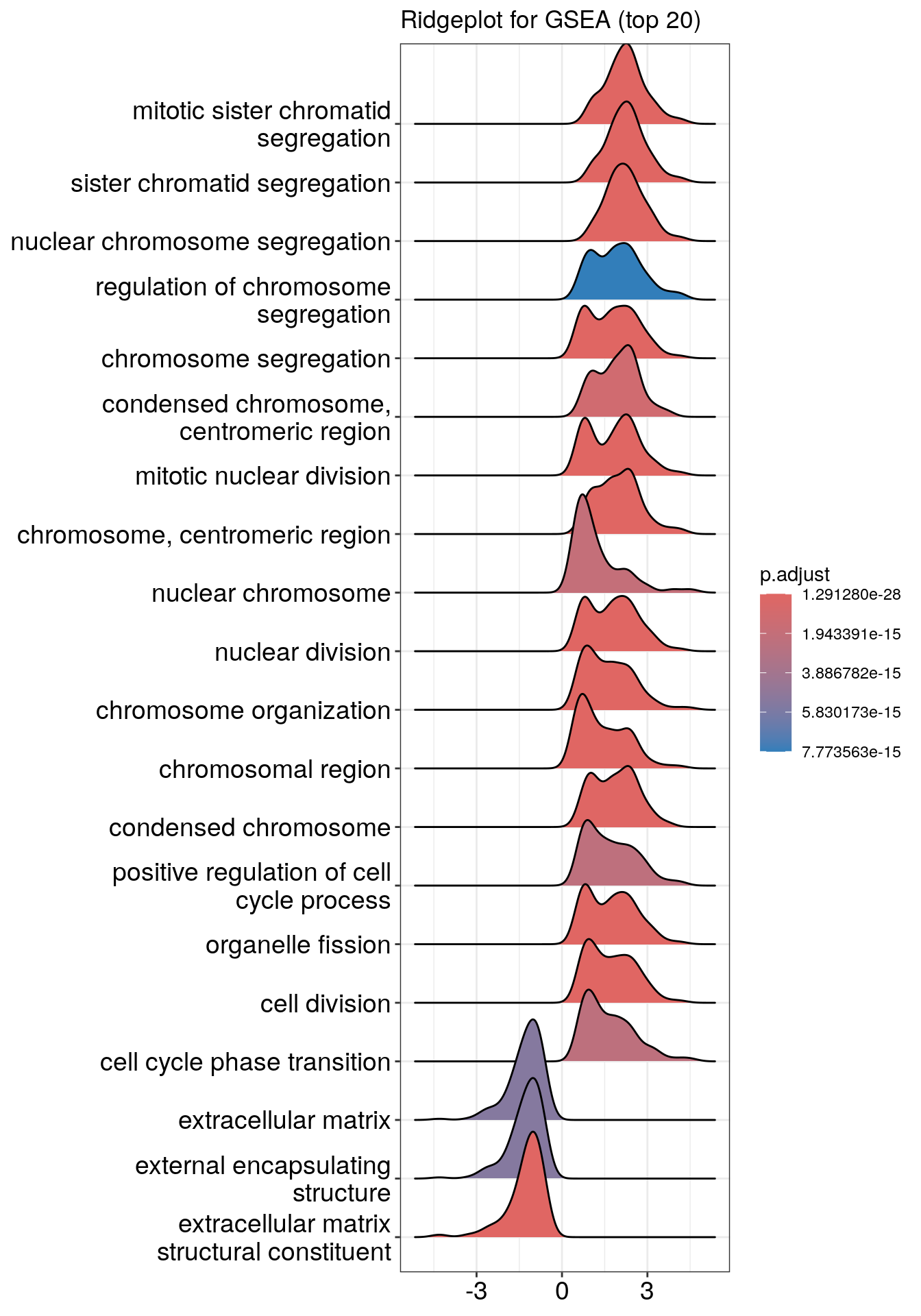

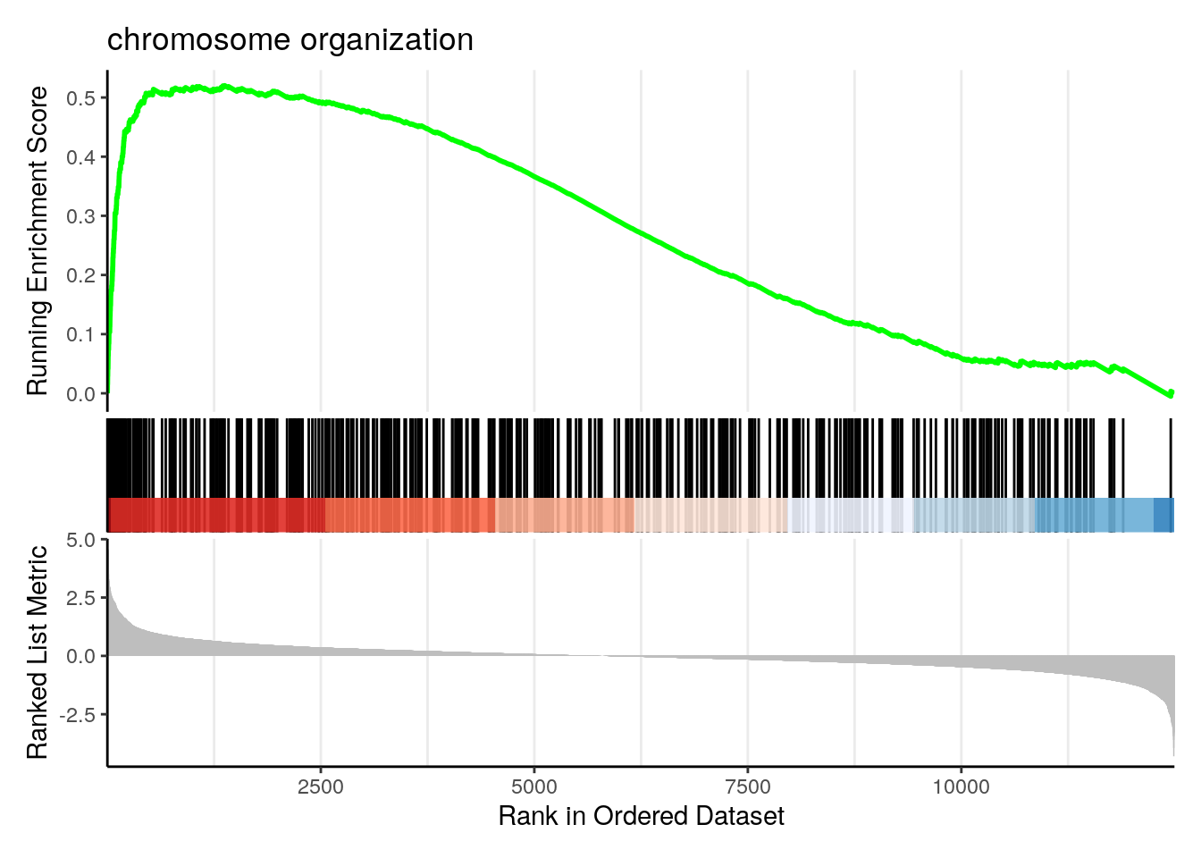
Running score and preranked list of GSEA result

Running score and preranked list are traditional methods for visualizing GSEA result. You are familiar with these visualisations from Module 2. The function gseaplot() supports visualising both the distribution of the gene set and the enrichment score.

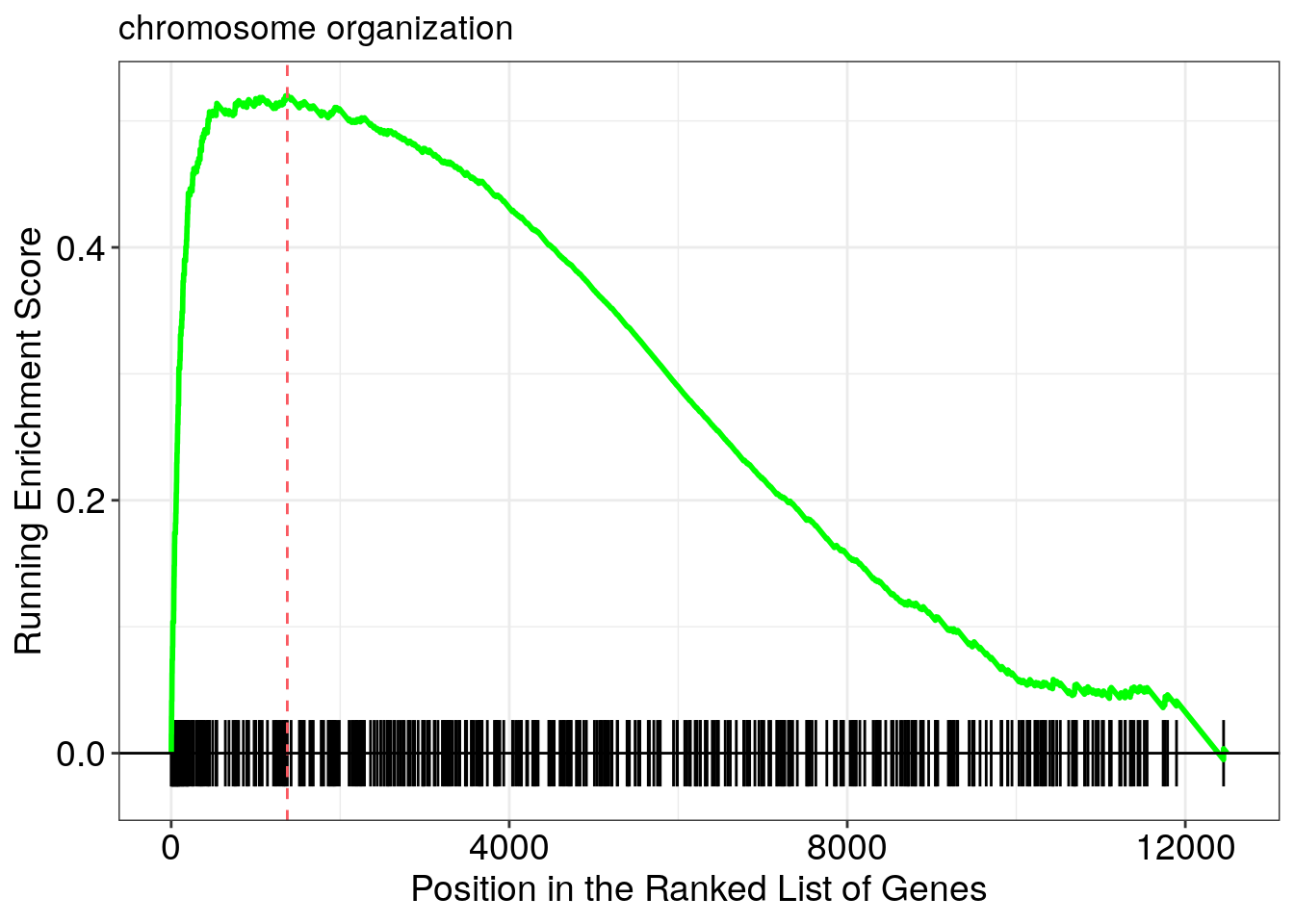
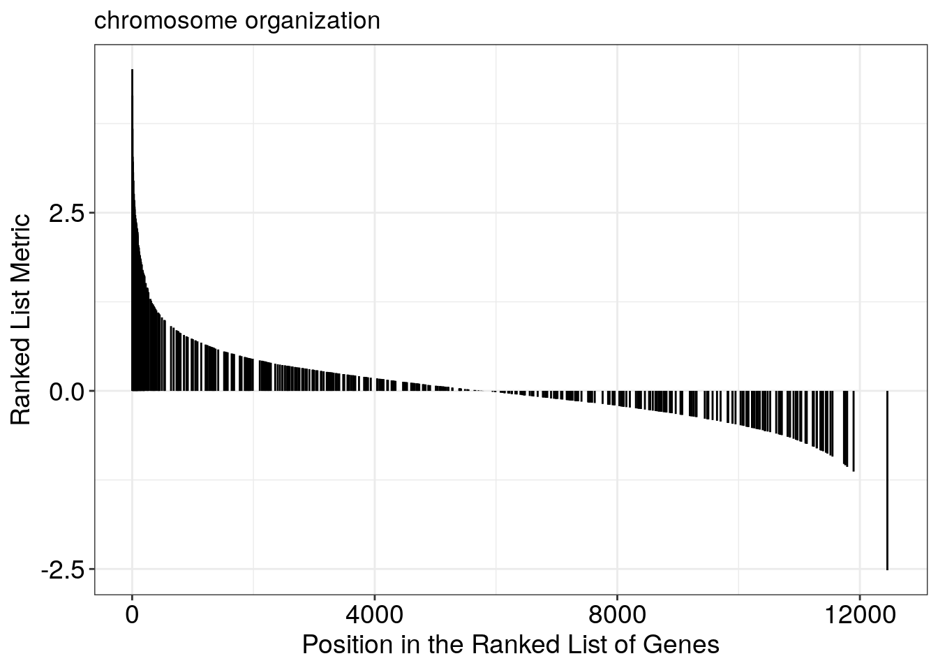
gseaplot(egsea, geneSetID = 1, by = "runningScore", title = egsea$Description[1])

gseaplot(egsea, geneSetID = 1, by = "preranked", title = egsea$Description[1])

Another method to plot GSEA result is the gseaplot2 function:

gseaplot2(egsea, geneSetID = 1, title = egsea$Description[1])

Enrichment Map

The function emapplot also supports visualising results of GSEA. As we did before, let us first calculate similarity using pairwise_termsim()

edo2 <- pairwise_termsim(egsea)
emapplot(edo2)+ ggtitle("GSEA Enrichment Map")

## Warning: ggrepel: 6 unlabeled data points (too many overlaps). Consider
## increasing max.overlaps

```

What next?

This figure gives a complete overview of functionalities of clusterProfiler

Explore other features of `clusterProfiler`

For other functionalities in clusterProfiler please refer to detailed examples in this book

Bonus - Try it yourself:

Using your knowledge of clusterProfiler, write scripts to perform the following analysis. Use the geneList dataset.

Run ORA against GO molecular function by converting gene to uniprot IDs
Run ORA against KEGG pathways, Reactome and Wikipathways databases
Run GSEA against KEGG pathways, Reactome and Wikipathways databases
Use your data to run ORA and GSEA using clusterProfiler

Hint: clusterProfiler provides different functions for testing against multiple databases. Refer the book for complete list.

Ontologies and pathway databases supported by `clusterProfiler`

Disease Ontology (via DOSE)
Network of Cancer Gene (via DOSE)
DisGeNET (via DOSE)
Gene Ontology (supports many species with GO annotation query online via AnnotationHub)
KEGG Pathway and Module with latest online data (supports more than 4000 species listed in http://www.genome.jp/kegg/catalog/org_list.html)
Reactome Pathway (via ReactomePA)
DAVID (via RDAVIDWebService)
Molecular Signatures Database
- hallmark gene sets
- positional gene sets
- curated gene sets
- motif gene sets
- computational gene sets
- GO gene sets
- oncogenic signatures
- immunologic signatures
Other Annotations
- from other sources (e.g. DisGeNET as an example)
- user’s annotation
- customized ontology
- and many others

All publications describing `clusterProfiler` can be found here:

T Wu^#, E Hu^#, S Xu, M Chen, P Guo, Z Dai, T Feng, L Zhou, W Tang, L Zhan, X Fu, S Liu, X Bo^*, G Yu^*. clusterProfiler 4.0: A universal enrichment tool for interpreting omics data. The Innovation. 2021, 2(3):100141. doi: 10.1016/j.xinn.2021.100141
G Yu^*. Gene Ontology Semantic Similarity Analysis Using GOSemSim. In: Kidder B. (eds) Stem Cell Transcriptional Networks. Methods in Molecular Biology. 2020, 2117:207-215. Humana, New York, NY. doi: 10.1007/978-1-0716-0301-7_11
G Yu^*. Using meshes for MeSH term enrichment and semantic analyses. Bioinformatics. 2018, 34(21):3766–3767. doi: 10.1093/bioinformatics/bty410
G Yu, QY He^*. ReactomePA: an R/Bioconductor package for reactome pathway analysis and visualization. Molecular BioSystems. 2016, 12(2):477-479. doi: 10.1039/C5MB00663E
G Yu^*, LG Wang, and QY He^*. ChIPseeker: an R/Bioconductor package for ChIP peak annotation, comparison and visualization. Bioinformatics. 2015, 31(14):2382-2383. doi: 10.1093/bioinformatics/btv145
G Yu^*, LG Wang, GR Yan, QY He^*. DOSE: an R/Bioconductor package for Disease Ontology Semantic and Enrichment analysis. Bioinformatics. 2015, 31(4):608-609. doi: 10.1093/bioinformatics/btu684
G Yu, LG Wang, Y Han and QY He^*. clusterProfiler: an R package for comparing biological themes among gene clusters. OMICS: A Journal of Integrative Biology. 2012, 16(5):284-287. doi: 10.1089/omi.2011.0118
G Yu, F Li, Y Qin, X Bo^*, Y Wu, S Wang^*. GOSemSim: an R package for measuring semantic similarity among GO terms and gene products. Bioinformatics. 2010, 26(7):976-978. doi: 10.1093/bioinformatics/btq064

Merkel, Dirk. 2014. “Docker: Lightweight Linux Containers for Consistent Development and Deployment.” Linux Journal 2014 (239): 2.

Optional Module 8 Lab 3: Automated Enrichment and Visualisation Lab using clusterProfiler

clusterProfiler lab

Goal

Supported Analysis

Install and load packages

Exercise 1a. Over representation analysis

Data for enrichment using clusterProfiler

Data for over representation analysis using clusterProfiler

Perform GO over representation analysis

Results of GO over representation analysis

Input options for enrichGO():

Simplify enrichGO() results

Exercise 1b. Visualise the results of GO over representation analysis

Barplot

Dotplot

Enrichment Map

Upset plot

Details about the input arguments for enrichGO()

A note on supported organisms

Exercise 2a: Gene set enrichment analysis

Data for running gene set enrichment analysis in clusterProfiler

Perform GO gene set enrichment analysis

Results of GO gene set enrichment analysis

Input options for gseGO()

Details about the input arguments for gseGO()

Exercise 2b. Visualise the results of gene set enrichment analysis

Dotplot

Ridgeline plot

Running score and preranked list of GSEA result

Enrichment Map

What next?

Explore other features of clusterProfiler

Bonus - Try it yourself:

Ontologies and pathway databases supported by clusterProfiler

All publications describing clusterProfiler can be found here:

Optional Module 8 Lab 3: Automated Enrichment and Visualisation Lab using `clusterProfiler`

`clusterProfiler` lab

Data for enrichment using `clusterProfiler`

Data for over representation analysis using `clusterProfiler`

Input options for `enrichGO()`:

Simplify `enrichGO()` results

Details about the input arguments for `enrichGO()`

Data for running gene set enrichment analysis in `clusterProfiler`

Input options for `gseGO()`

Details about the input arguments for `gseGO()`

Explore other features of `clusterProfiler`

Ontologies and pathway databases supported by `clusterProfiler`

All publications describing `clusterProfiler` can be found here: