Module 3 Lab: (Bonus) Automation
This work is licensed under a Creative Commons Attribution-ShareAlike 3.0 Unported License. This means that you are able to copy, share and modify the work, as long as the result is distributed under the same license.
By Ruth Isserlin
Although a lot of what we have demonstrated in Cytoscape up until now has been manual most of the features we use can be automated through multiple access points including:
- R/Rstudio using RCy3 - a bioconductor package that makes communicating with cytoscape as simple as calling a method.
- Python using py2cytoscape.
- directly through cyrest using rest calls - you can use any programming language with the rest API. See Cytoscape Automation
Automation becomes helpful when performing pipelines multiple times on similiar datasets or integrating cytoscape data into your other pipelines.
Below we demonstrate how to perform the enrichment map pipeline from R but automation is not limited to this access point. You can automate it from any flavour of programming.
Check out all the ways you can interact with Cytoscape here including directly through the cytoscape command window.
Goal of the exercise:
Run an enrichment analysis and Create an enrichment map automatically from R/Rstudio
During this exercise, you will apply what you have learnt in Module 2 labs and Module 3 labs but instead of performing them manually you will automate the process using R/Rstudio. We will use all the same data and programs we used in the previous labs but we will control them from R.
Before starting this exercise you need to set up R/Rstudio. You can do that directly on your machine or through docker.
Set Up - Option 1 - Install R/Rstudio
- Install R.
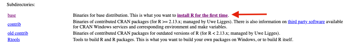
- Go to: https://cran.rstudio.com/
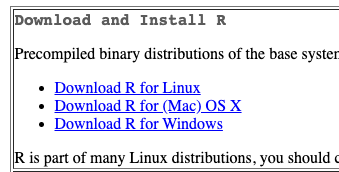
- If installing on Windows select “install R for the first time” to get to the required package.
RStudio is a free IDE (Integrated Development Environment) for R. RStudio is a wrapper1 for R and as far as basic R is concerned, all the underlying functions are the same, only the user interface is different (and there are a few additional functions that are very useful e.g. for managing projects).
Here is a small list of differences between R and RStudio.
pros (some pretty significant ones actually):
- Integrated version control.
- Support for “projects” that package scripts and other assets.
- Syntax-aware code colouring.
- A consistent interface across all supported platforms. (Base R GUIs are not all the same for e.g. Mac OS X and Windows.)
- Code autocompletion in the script editor. (Depending on your point of view this can be a help or an annoyance. I used to hate it. After using it for a while I find it useful.)
- “Function signaturtes” (a list of named parameters) displayed when you hover over a function name.
- The ability to set breakpoints for debugging in the script editor.
- Support for knitr, and rmarkdown; also support for R notebooks … (This supports “literate programming” and is actually a big advance in software development)
- Support for R notebooks.
cons (all minor actually):
- The tiled interface uses more desktop space than the windows of the R GUI.
- There are sometimes (rarely) situations where R functions do not behave in exactly the same way in RStudio.
- The supported R version is not always immediately the most recent release.
- Navigate to the RStudio download Website.
- Find the right version of the RStudio Desktop installer for your computer, download it and install the software.
- Open RStudio.
-
Focus on the bottom left pane of the window, this is the “console” pane.
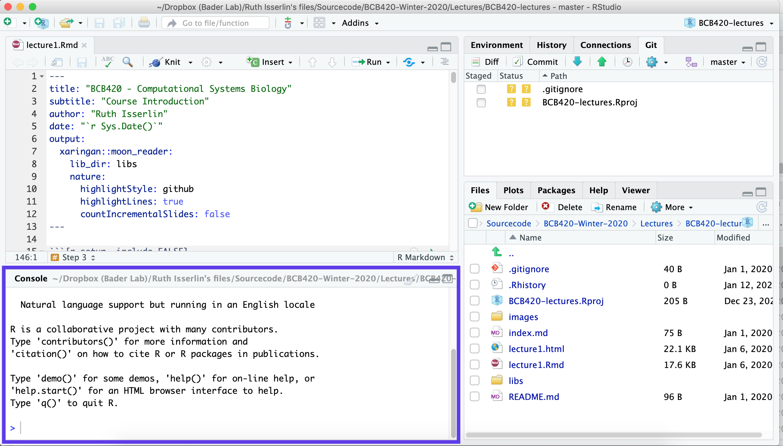
- Type getwd().
- This prints out the path of the current working directory. Make a (mental) note where this is. We usually always need to change this “default directory” to a project directory.
Set Up - Option 2 - Docker image with R/Rstudio
Changing versions and environments are a continuing struggle with bioinformatics pipelines and computational pipelines in general. An analysis written and performed a year ago might not run or produce the same results when it is run today. Recording package and system versions or not updating certain packages rarely work in the long run.
One the best solutions to reproducibility issues is containing your workflow or pipeline in its own coding environment where everything from the operating system, programs and packages are defined and can be built from a set of given instructions. There are many systems that offer this type of control including:
“A container is a standard unit of software that packages up code and all its dependencies so the application runs quickly and reliably from one computing environment to another.” (???)
Why are containers great for Bioiformatics?
- allows you to create environments to run bioinformatis pipelines.
- create a consistent environment to use for your pipelines.
- test modifications to the pipeline without disrupting your current set up.
- Coming back to an analysis years later and there is no need to install older versions of packages or programming languages. Simply create a container and re-run.
What is docker?
- Docker is a container platform, similar to a virtual machine but better.
- We can run multiple containers on our docker server. A container is an instance of an image. The image is built based on a set of instructions but consists of an operating system, installed programs and packages. (When backing up your computer you might taken an image of it and restored your machine from this image. It the same concept but the image is built based on a set of elementary commands found in your Dockerfile.) - for overview see here
- Often images are built off of previous images with specific additions you need for you pipeline. (For example, for this course we use a base image supplied by bioconductorrelease 3.11 and comes by default with basic Bioconductor packages but it builds on the base R-docker images called rocker.)
Docker - Basic term definition
Container
- An instance of an image.
- the self-contained running system.
- There can be multiple containers derived from the same image.
Image
- An image contains the blueprint of a container.
- In docker, the image is built from a Dockerfile
Docker Volumes
- Anything written on a container will be erased when the container is erased ( or crashes) but anything written on a filesystem that is separate from the contain will persist even after a container is turned off.
- A volume is a way to assocaited data with a container that will persist even after the container. * maps a drive on the host system to a drive on the container.
- In the above docker run command (that creates our container) the statement:
- maps the directory ${PWD} to the directory /home/rstudio/projects on the container. Anything saved in /home/rstudio/projects will actually be saved in ${PWD}
- An example:
- I use the following commmand to create my docker container:
docker run -e PASSWORD=changeit --rm \
  -v /Users/risserlin/code:/home/rstudio/projects \
  -p 8787:8787 \
risserlin/workshop_base_image- I create a notebook called task3.Rmd and save it in /home/rstudio/projects.
Note: Do not save it in /home/rstudio/ which is the default directory RStudio will start in
- On my host computer, if I go to /Users/risserlin/code I will find the file task3.Rmd
Install Docker
- Download and install docker desktop.
- Follow slightly different instructions for Windows or MacOS/Linux
Windows
- it might prompt you to install additional updates (for example - https://docs.Microsoft.com/en-us/windows/wsl/install-win10#step-4---download-the-linux-kernel-update-package) and require multiple restarts of your system or docker.
- launch docker desktop app.
- Open windows Power shell
- navigate to directory on your system where you plan on keeping all your code. For example: C:\USERS\risserlin\code
- Run the following command: (the only difference with the windows command is the way the current directory is written. ${PWD} instead of "$(pwd)")
docker run -e PASSWORD=changeit --rm \
  -v ${PWD}:/home/rstudio/projects -p 8787:8787 \
  risserlin/workshop_base_image
- Windows defender firewall might pop up with warning. Click on Allow access.
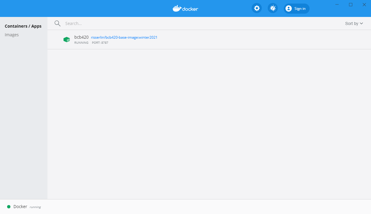
- In docker desktop you see all containers you are running and easily manage them.
MacOS / Linux
- Open Terminal
- navigate to directory on your system where you plan on keeping all your code. For example: /Users/risserlin/code
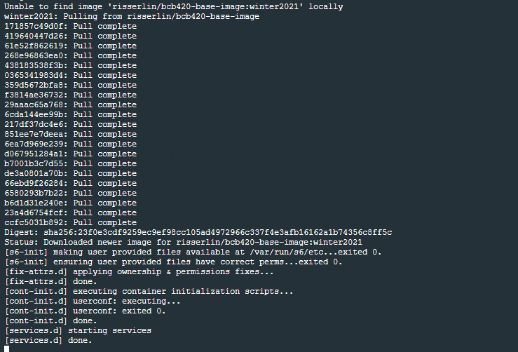
- Run the following command: (the only difference with the windows command is the way the current directory is written. ${PWD} instead of "$(pwd)")
docker run -e PASSWORD=changeit --rm \
  -v "$(pwd)":/home/rstudio/projects -p 8787:8787 \
  risserlin/workshop_base_image
Create your first notebook using Docker
Start coding!
- Open a web browser to localhost:8787
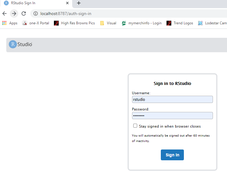
- enter username: rstudio
- enter password: changeit
- changing the parameter -e PASSWORD=changeit in the above docker command will change the password you need to specify
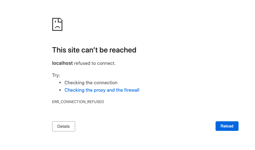
- Make sure your docker container is running. (If you rebooted your machine you will need to restart the container on reboot.)
- Make sure you got the right port.
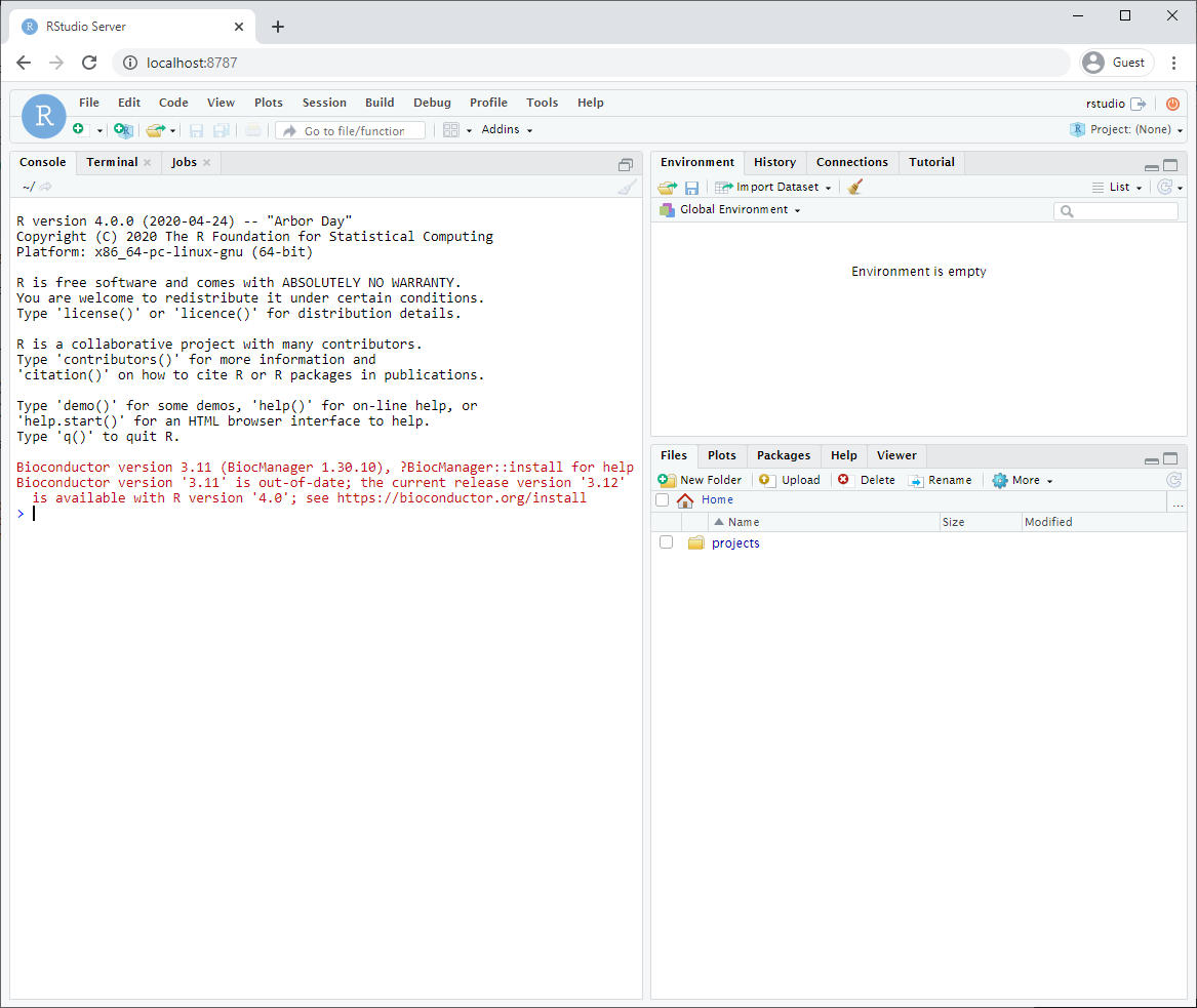
After logging in, you will see an Rstudio window just like when you install it directly on your computer. This RStudio will be running in your docker container and will be a completely separate instance from the one you have installed on your machine (with a different set of packages and potentially versions installed).
Make sure that you have mapped a volume on your computer to a volume in your container so that files you create are also saved on your computer. That way, turning off or deleting your container or image will not effect your files.
- The parameter -v ${PWD}:/home/rstudio/projects maps your current directory (i.e. the directory you are in when launching the container) to the directory /home/rstudio/projects on your container.
- You do not need to use the ${PWD} convention. You can also specify the exact path of the directory you want to map to your container.
- Make sure to save all your scripts and notebooks in the projects directory.
- Create your first notebook in your docker Rstudio.
- Save it.
- Find your newly created file on your computer.
Start using automation
- Download example R notebooks from https://github.com/BaderLab/Cytoscape_workflows.
This repository contains example R Notebooks that automate the enrichment map pipeline.
There are two ways you can download this collection:
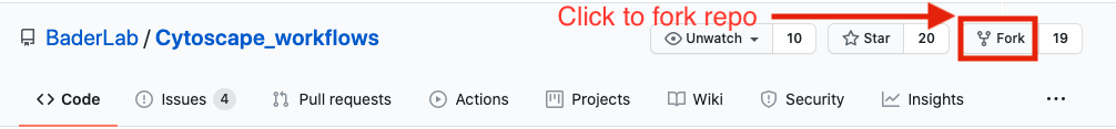
- If you are familiar with git then we recommend you fork the repo and use it like you would use any github repo.
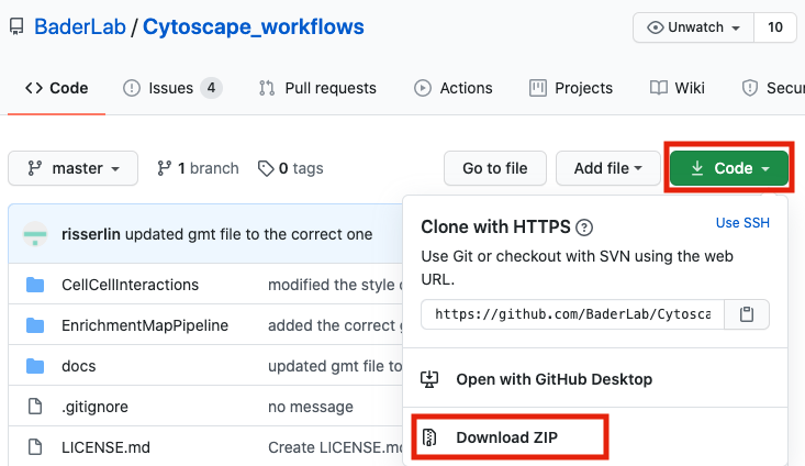
- download the collection as a zip file - unzip folder and place in CBW working directory
If you are new to git and want to learn more about code versioning then we recommend you read the following tutorial And check out Github Desktop - a desktop application to communicate with github.
Step 1 - launch RStudio
- Launch RStudio by double clicking on the installed program icon.
Step 2 - create a new project
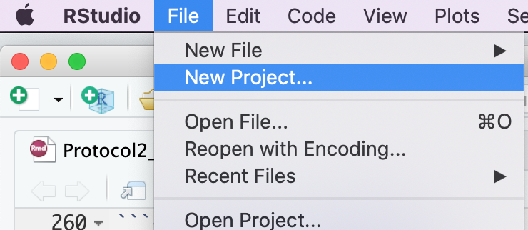
- Create a new project - File -> New R Project …
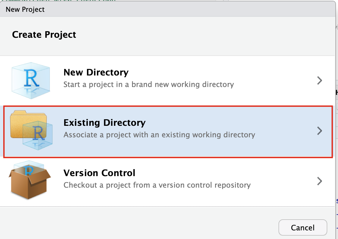
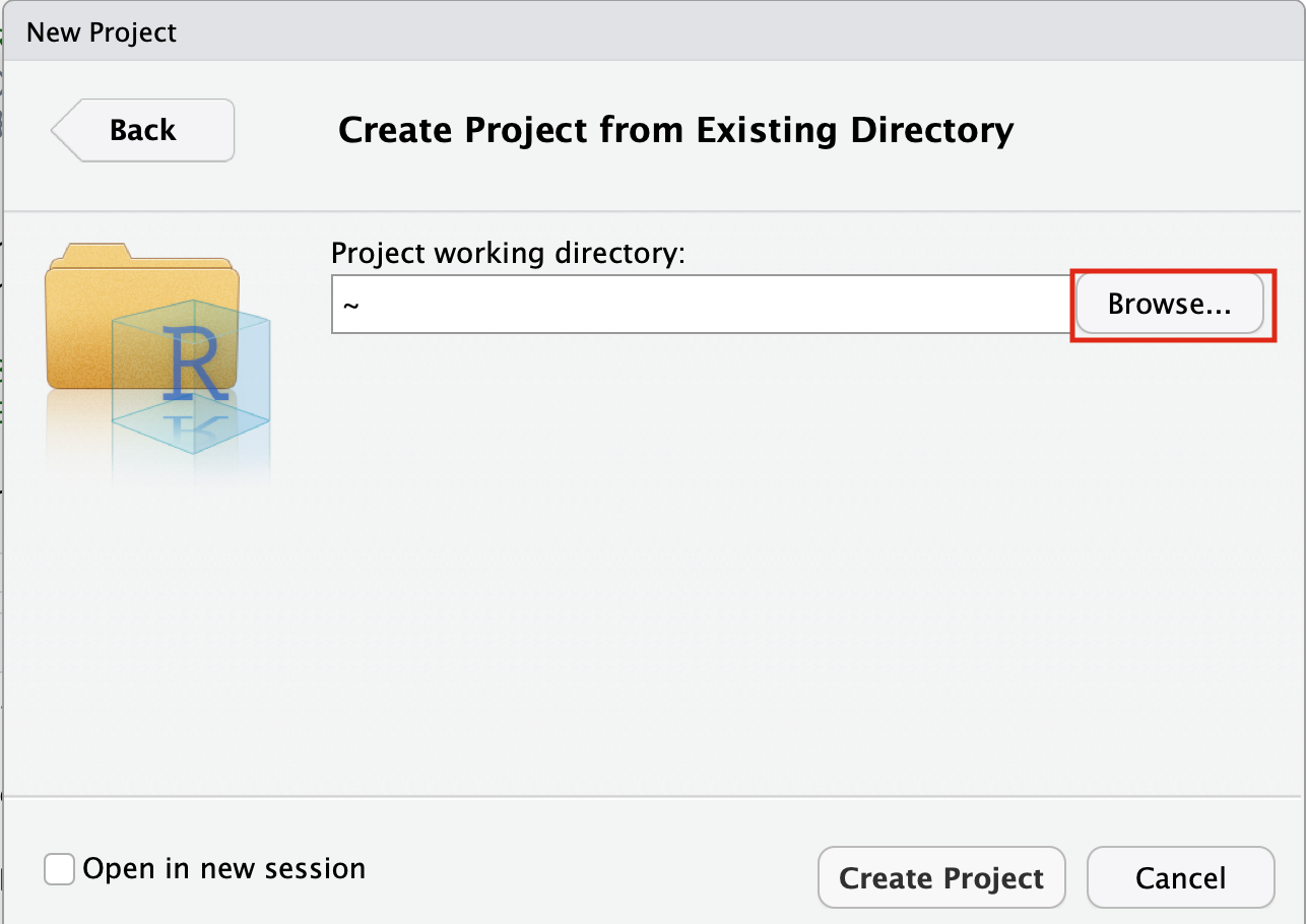
- Select Create project from - “Existing Directory”
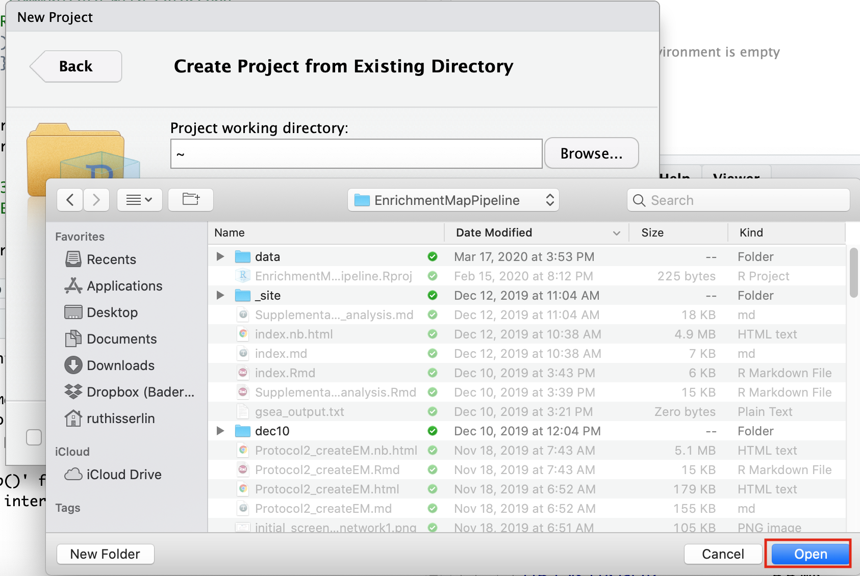
- Click on the Browse button
- Navigate to the EnrichmentMapPipeline directory that is found in the directory you downloaded and unzipped from github. (for example, if it is still in your downloads directory go to ~/Downloads/Cytoscape_workflows/EnrichmentMapPipelines)
Step 3 - Open example up RNotebook
Open the RNotebook Protocol2_createEM.Rmd
Go to File –> Open File …
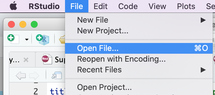
Click on Protocol2_createEM.Rmd
If the file is not found in the first directory that RStudio opens up then go back and make sure that you created an Rproject from an “Existing directory” in the previous step.
Step 4 - Define Notebook parameters
Setting up Notebooks with parameters allows you to re-run the same notebook with different datasets very easily. Whereever possible create notebooks with parameters so you can re-use them
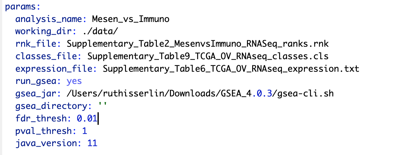
Descriptions of each of the parameters:
- analysis_name - change this field to whatever you want your analysis to be called. GSEA directories generated will be named using this string. It will have additional characters added to it as GSEA generates a random number that it associates with each of its output directories.
- working_dir - path to directory containing the data files we will be analyzing.
- rnk_file - NOT Optional. This notebook runs GSEA preranked and this is the only file that is required. for details on the specifications of this file see Module 3 - gsea lab.
- class_file - (Optional) this file is a GSEA specific data file and is used for better visualization in the heat map viewer of enrichment map. For details of the creation of this file see - GSEA documentation - class files
- expression_file - (Optional) this file contains the expression values for each of the experiments used in to create your rank file. It is used for better visualization in the heat map viewer of enrichment map.
- run_gsea - set to yes or no. This variable specifies whether the notebook should run GSEA. GSEA can take a while to run so if you have already performed the GSEA analysis and simply want to create an enrichment map you can set this variable to “no”. If this variable is set to no then you need to specify the path and the name of the GSEA directory in “gsea_directory” parameter.
- gsea_jar - full path to the gsea jar. In the latest version of GSEA this is actually a bat(for windows users) or a sh (for moc and linux users) script. If using GSEA 3.0 or older set this variable to the full path to the gsea.jar We do not recommend using GSEA 3.0 or older versions
- gsea_directory - full path to gsea results directory. Only populate if run_gsea is set to “no”.
- fdr_threshold - FDR threshold used to create enrichment map
- pval_thresho - pvalue threshold used to create enrichment map
- java_version - for backwards compatibility. For users using previous version of GSEA and older versions of java.
For this initial analysis change:
- gsea_jar - change to the full path to the gsea jar that you were instructed to download in your pre-workshop setup instructions
This is not the same as the GSEA application that we used in Module 2 gsea lab. 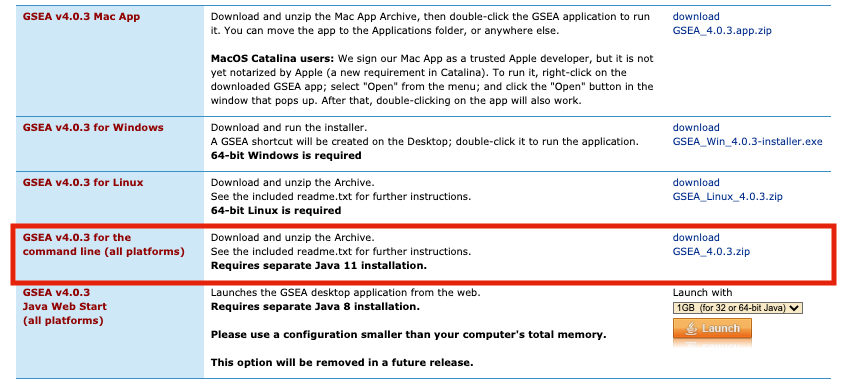
If you are using the docker implementation GSEA is already in the docker and you don’t need to downlaod anything else. Just set this parameter as:
gsea_jar: /home/rstudio/GSEA_4.1.0/gsea-cli.sh
Step 5 - Step through notebook to run the analysis
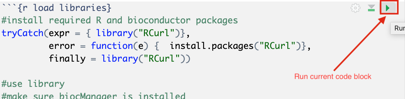
The RNotebook is a mixture of markdown text and code blocks.
Read through the notebook to understand what each section is doing and sequentially run the code blocks by clicking on the play button at the top right of each code block.
Exercises
Once you have run through the notebook and created your enrichment map automatically try the following:
- change the fdr threshold and create a new network (without rerunning the whole notebook) with the lower FDR threshold.
- change the similarity coeffecient and create a new network (without rerunning the whole notebook) with the lower FDR threshold.
- re-run the notebook using the GSEA results you created on the first run without running GSEA.
- Modify notebook to run with a different gmt file. (Downloaded from somewhere else or a different file found on baderlab genesets download site)
- Open the notebook Supplementary_Protocol5_Multi_dataset_theme_analysis.Rmd and run through it to create a multi dataset enrichment map.
Additional resources
Check out all the different notebooks available here
A “wrapper” program uses another program’s functionality in its own context. RStudio is a wrapper for R since it does not duplicate R’s functions, it runs the actual R in the background.↩︎